In my first pass at text analysis of the ESA program, I looked at how the frequency of words used in the ESA program differed from last year to this year. There are much more sophisticated ways at looking at word use in text, though, and I began to dive into the text-mining literature to find other ways to draw insight from ESA abstracts.
One method I found is topic modeling using latent Dirichlet allocation (LDA). Using this method, a number of “topics” are identified, each consisting of groups of words occur together. Documents are treated as linear mixtures of these topics. Carson Sievert recently wrote a great blog post on the ROpenSci blog about this and his package with Kenneth E. Shirley, LDAvis, which produces interactive visualizations of of LDA models.
I had trouble wrapping my head around LDA at first, but on Wednesday at ESA, Dave Harris alerted me to an awesome talk by Denis Valle. Valle showed that LDA can be used to model assemblages of species. In this case, we model communities of co-occurring species, rather than topics of co-occurring words, and rather than documents, we have sample locations. He demonstrated the method on USFS Forest Inventory and Analysis data, showing distinct communities of trees in Eastern U.S. forests. Valle’s talk made LDA much clearer to me, and showed that LDA could be an alternative to other methods of community analysis such as ordination. I’m looking forward to the forthcoming paper.
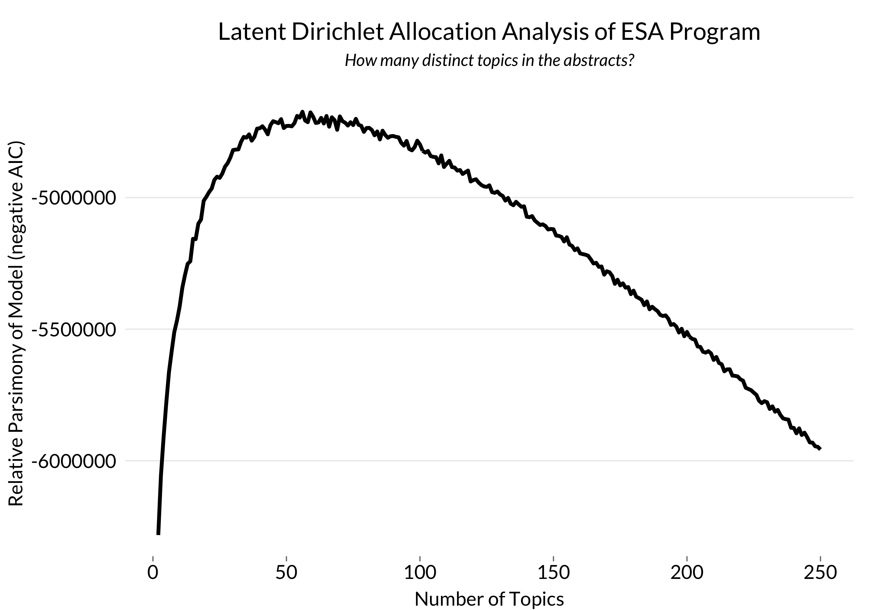
Back to the ESA program: LDA requires that we specify the number of topics, and it then allocates words among those topics. So I fit a series of models and used AIC to determine the best fit:

The model with the lowest AIC breaks the ESA program into 56 different topics. We can explore this model with an interactive visualization created by LDAvis:
On the left, topics are represented as numbered circles, with the number representing their rank (1 = most common topic), and their size representing relative frequency across all abstracts. They are plotted so that similar topics are clustered together and different topics are farther apart.
Click on any circle and you’ll see a list of the top 30 terms making up that topic on the right. Note that the words are “stemmed” - their suffixes have been removed so as to treat different forms of the same word as a single value. Relative word ranking is a balance between the importance of the word within the topic (red bars) and the frequency of the word across all documents (grey bars). You can adjust this balance using the ‘Lambda’ box on the top-right. Click on any word and you’ll see in what other topics it appears.
Let’s explore! Clicking on Topic 1, we see very general words that might appear in any abstract. Topic 2 seems to be made up of words related to conservation and planning, showing the importance of this subject in the meeting. But click on “cost” in Topic 2 and you’ll see that this term is important in several other topics: 23 (words involving life-history), 36 (plant-water relations), and 47 (behavioral ecology). Topic 3 consists of general words having to do with methods, but nearby, topics 10 and 11 consist of words related to data collection and modeling, respectively.
One interesting observation is that “California” is most frequent in Topic 42, which consists of words related to marine systems, and is also common in 53 (invasions), 38 (fire), and 36 (plant-water relations). I was unsurprised at the last two (especially given fire’s importance in my last analysis), but hadn’t realized how California-specific marine topics would be.
There’s lots more to explore here, though it’s not always easy to interpret. Some topics seem to map well to ecological sub-fields, while others may be driven by concepts and frameworks that are difficult to classify, or even writing style. What patterns do you see that are worth a harder look?
Code for this analysis is on Github here.